Equations of Motion by Graphical Method

Introduction to Equations Of Motion
In this article, we will learn how we can relate quantities like velocity, time, acceleration and displacement provided the acceleration remains constant. These relations are collectively known as the equation of motion. There are three equations of motion. There are three ways to derive the equation of motion and here we are going to derive with the help of a graph.

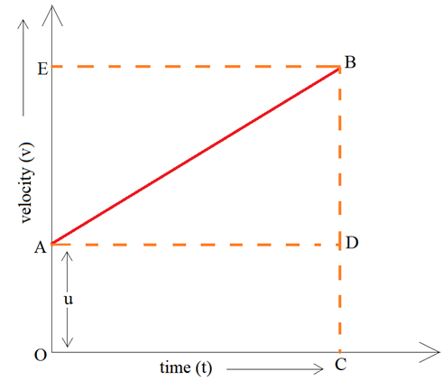
First Equation of Motion
First equation of motion relates velocity, time and acceleration. Now in ∆uxy,
We also know that tanθ is nothing but the slope, and slope of the v – t graph represents acceleration.
⇒ v = u + at ———– (1)
This is the first equation of motion where,
v = final velocity
u = initial velocity
a = acceleration
t = time taken

Second Equation of Motion
Now coming to the second equation of motion, it relates displacement, velocity, acceleration and time. The area under the v – t graph represents the displacement of the body.
In this case,
Displacement = Area of the trapezium (ouxt)
We can substitute v in terms of others and get the final equation as:
Where symbols have their usual meaning.

Third Equation of Motion
The third equation of motion relates to velocity, displacement, and acceleration. Using the same equation (2),
Using equation (1), if we replace t, we get,
The above equation represents our third equation of motion.

Applications of Equations of Motion
So now that we have seen all three equations of motion, we can use them to solve kinematic problems. We just have to identify what all parameters are given and then choose the appropriate equation and solve for the required parameter. The equations of motion are also used in the calculation of optical properties.